Note: this post makes heavy use of MathJax. If you're reading via RSS,
you'll want to click through to the web version.
My intuition of
regularization is:
it's a compromise. You want a model that fits your historical examples, but you
also want a model that is "simple." So you set some exchange rate -- the
strength of regularization -- and trade off "fit my historical data" against "be
a simple model." You meet somewhere in the middle: a model that's simpler than
your unregularized fit would produce, but not so simple to the point that it's
missing obvious/reliable patterns in the training data.
In the biz, we call it a penalty on complexity, which is different than calling
it a ban on complexity. We call it shrinking, which is different than calling
it vanishing. These names reflect the intuition: penalize something to get
less of it, but not none of it; shrink something to make it smaller, not
to make it disappear. With regularization, we'll reach some compromise point,
and get a model that (a) is less well-fit to the training data than in the
unregularized state, but also (b) not maximally, uselessly "simple."
This blog post is about how the world's most famous regression scheme,
the Lasso (Tibshirani 1996), rejects
compromise. For certain, sufficiently-high penalty rates, it will quite happily
only give you a maximally-simple model: one that zeros out consideration of
any predictive features you handed it. No compromise, just an all-zeros empty
model; "I found no pattern in the data." And people love this about the Lasso!
My dissertation
was built on this property, where Lasso regularization can zero out model
weights.
But it's also weird to me that it's possible, given what I thought we were doing
by regularizing a model fit. It's not a compromise anymore.
Why's Lasso do that?
What's Lasso? (A convex optimization.)
It's typical for statisticians to formalize "fit the data, but with a simple
model" by posing an optimization task built on five raw ingredients:
- Defining "the data" as a collection of \(N\) examples, represented as
vector-scalar pairs, \(\left\{\vec{\mathbb{x}}_j, y_j\right\}_{j = 1}^N\)
Each \(\vec{\mathbb{x}}_j\) is in \(\mathbb{R}^p\) (call each of these an
example's feature vector) and each \(y_j\) is an example's scalar label.
- Defining the model as a vector of \(p\) parameters,
\(\vec{\mathbb{w}} \in \mathbb{R}^p\). Call each individual parameter (i.e.,
each vector element \(w_i,~i = 1, \ldots, p\)), a model weight.
- Defining a function,
\(f\left(~\cdot~; \left\{\vec{\mathbb{x}}_j, y_j\right\}_{j = 1}^N\right): \mathbb{R}^p \to \mathbb{R}\),
that expresses goodness-of-fit. By construction of \(f\), a model parameter
vector that minimizes \(f\) corresponds to a model that's "fitting the data"
to the best possible extent. Call \(f\) the loss function.
- Defining a function, \(r: \mathbb{R}^p \to \mathbb{R}\), that expresses
model simplicity. A model parameter vector that minimizes this function
corresponds to a maximally simple model. Call \(r\) the regularizer.
- Defining a scalar hyperparameter, \(\lambda \geq 0\), that defines the
strength of regularization. The bigger \(\lambda\), the more we favor \(r\)
over \(f\).
Mixing these together, our optimization task is:
$$\vec{\mathbb{w}}^*(\lambda) := \arg \min_{\vec{\mathbb{w}} \in \mathbb{R}^p} f\left(\vec{\mathbb{w}}; \left\{\vec{\mathbb{x}}_j, y_j\right\}\right) + \lambda r(\vec{\mathbb{w}})$$
Lasso's loss function
Our loss function is defined as:
$$f\left(\vec{\mathbb{w}}; \left\{\vec{\mathbb{x}}_j, y_j\right\}_{j = 1}^N\right) = \sum_{j=1}^N{\left(\vec{\mathbb{w}}^T\vec{\mathbb{x}}_j - y_j\right)^2}$$
That's:
- the sum, over the features-and-label pairs for all \(N\) examples,
- of the square
- of the difference
- between the actual label \(y_j\)
- and the dot product of \(\vec{\mathbb{w}}\) and \(\vec{\mathbb{x}}_j\)
The model weights "fit the data" by producing a weighted sum of the example's
features that is a reliably close match to the example's scalar label.
The loss function is a sum of squares, so it's always non-negative. The closer
it is to zero, the better the average label match we are getting from our model
weights. Minimize the loss function to best fit the data, just how we wanted.
Lasso's regularizer
Our regularizer is:
$$r\left(\vec{\mathbb{w}}\right) = \left|\left|\vec{\mathbb{w}}\right|\right|_1 = \sum_{i=1}^p\left|w_i\right|$$
the \(L_1\) norm of our model weight vector. Models with weights that are
reliably close to zero count as "simpler" than ones with larger-magnitude
weights. Just like \(f\), \(r\) is always non-negative. We can minimize it by
choosing a weight vector of all zeroes. The model that always picks "zero" as
its guess for \(y\), totally ignoring the example's features, is this
regularizer's simplest possible model.
Lasso's convexity
Altogether, the optimization task is:
$$\vec{\mathbb{w}}^*(\lambda) := \arg \min_{\vec{\mathbb{w}} \in \mathbb{R}^p} f\left(\vec{\mathbb{w}}; \left\{\vec{\mathbb{x}}_j, y_j\right\}\right) + \lambda r(\vec{\mathbb{w}})$$
Take on faith that this mixture of \(f\), \(r\), and \(\lambda\) is convex.
\(f\) and \(r\) are both convex, and \(\lambda\) is non-negative, which lets us argue
- the scaling-up of a convex function by a non-negatve value is itself convex,
so \(\lambda r(\vec{\mathbb{w}})\) is also convex,
- the sum of two convex functions is itself convex, so the overall mixture
\((f + \lambda r)\) we're minimizing is convex.
Convex functions come with a lot of nice properties I will leverage later on, so
I want to emphasize the convexity of our optimization task now.
Dropping down to univariate Lasso
At this point, we'll take a special case: when \(p\) is 1. This univariate
regression means both (a) our weight and (b) each example's feature "vector",
are just plain ol' scalars. Our optimization task, with \(w \in \mathbb{R}\)
and \(x_j \in \mathbb{R}\):
$$w^*(\lambda) := \arg \min_{w \in \mathbb{R}} \sum_{j=1}^N{\left(w \cdot x_j - y_j\right)^2} + \lambda\left|w\right|$$
I promise we're reinflate this to the multivariate case before we're done.
Lasso's convexity will help a lot with that.
But now that we're down here, we celebrate that low dimensionality means we can
make charts. Charts!
Here's a dataset with a clear relationship between \(x\) and \(y\). The data are
plotted as blue dots. I fit three Lasso models to this dataset, with \(\lambda\)
taking on values of 0, 350, or 800. I overlay the dashed trendlines each model
produces for the range of \(x\)'s, and we see those three trendlines decay from
a slope of 1 to a totally null (maximally simple!) slope of zero:

- The model with least regularization, \(\lambda = 0\) in blue, has a trendline
that best fits the data.
- The purple line, \(\lambda = 350\), is not a great fit to the data, but at
least is directionally correct when it identifies a positive correlation
between the example feature \(x\) and the example label \(y\).
- The red line, \(\lambda = 800\), totally ignores \(x\) and always predicts that
\(y\) is zero. This is what you get when \(w^*\) is maximizing \(r\) with no
regard for \(f\).
If we repeatedly produce a model weight \(w^*(\lambda)\) for many more values of
\(\lambda\), we can see this decay evolve in more detail (with our three models
above appearing as special large dots):
As regularization strength increases, the resulting model weight drops linearly,
until it hits absolute zero. Early on, you see compromise between \(f\) and \(r\):
\(f\) wants a slope of 1, and \(r\) wants a slope of 0, and as we strengthen \(r\)'s
negotiating leverage, we get models that look more and more like what \(r\) wants.
Not entirely what \(r\) wants: we still pick up on the positive correlation that
lives in the data. We don't discard \(f\)'s fit-the-data contributions entirely.
But past \(\lambda \approx 630\) or so (spoiler: I give you the exact formula for
this breakpoint a few sections from now), the optimization is ignoring the \(f\)
completely. That fit-the-data component is still there as part of the objective
to be minimized, and yet there's no compromise: the model weight returns what
\(r\) wants, and only what \(r\) wants. It's like \(f\) isn't even there, except it
is. We never zero'ed \(f\), we just amp'ed up \(r\).
What's Lasso doing? Why's Lasso do that?
What's Lasso doing? (Parabolas.)
Lasso is making our optimizer follow the instructions of a pair of parabolas.
When we strengthen regularization past a certain point, we're not able to make
either parabola happy, and bounce back and forth between them until we're stuck
at \(w^* = 0\).
Zero regularization
When there's no regularization at all, at \(\lambda = 0\), our optimizer's
objective is just to minimize the loss function \(f\), the sum of squared errors:
$$\begin{align}w^*(0) &= \arg \min_{w \in \mathbb{R}^p} f\left(w; \left\{x_j, y_j\right\}\right)\\
&= \arg \min_{w \in \mathbb{R}} \sum_{j=1}^N{\left(wx_j - y_j\right)^2}\end{align}$$
If we rearrange \(f\)'s terms a bit, we'll see it's a parabola as a function of
\(w\):
$$\begin{align}f\left(w; \left\{x_j, y_j\right\}\right) &= \sum_{j=1}^N{\left(wx_j - y_j\right)^2}\\
&= \sum_{j=1}^N \left[x_j^2 w^2 - 2 x_j y_j w + y_j^2\right] \\
&= \left[\sum_{j=1}^N x_j^2\right] w^2 - 2\left[\sum_{j=1}^N (x_j y_j)\right] w + \left[\sum_{j=1}^N y_j^2\right]\end{align}$$
Define some helpful aliases for those terms,
$$S_x := \sum_{j=1}^N x_j^2~~~~D_{xy} := \sum_{j=1}^N (x_j y_j)~~~~S_y := \sum_{j=1}^N y_j^2$$
where \(S\)'s stand for sums of squares our features or labels and \(D\) stands for
a dot product of feature and label. That makes the parabolaness of the
unregularized loss function really stand out:
$$f\left(w; \left\{x_j, y_j\right\}\right) = S_xw^2 - 2D_{xy}w + S_y$$
The vertex of a parabola like this lies at the famous "\(-b/2a\)" point, which
means \(f\) is minimized at:
$$w^*(0) = \frac{-(-2D_{xy})}{2S_x} = \frac{D_{xy}}{S_x}$$
(Or, expanding those terms for the fun of it:)
$$w^*(0) = \frac{\sum_{j=1}^N (x_j y_j)}{\sum_{j=1}^N x_j^2}$$
Let's plot \(f\left(w; \left\{x_j, y_j\right\}\right)\) for the blue-dots dataset
we used above:
We use an optimization routine that implements some kind of descent method to
start with any arbitrary guess at the \(w\) that minimizes \(f\), then refines it
until it finds the actual minimum. Imagine this optimization routine as a
little guy, wandering back and forth along the range of \(w\) to minimize \(f\).
Lasso's loss function parabola gives our little optimizer guy unambiguous
instructions:
Wherever you are right now, move towards \((D_{xy}/S_x)\). As long as each step
puts you lower than you were before, you will find the minimum.
If the little optimizer guy loops that enough, he'll land at \(w^*(0)\).
Some regularization
When we increase \(\lambda\) to some positive value, we're adding \(\lambda r(w)\)
to the function we want our little optimizer guy to minimize. That scaled
regularizer is a function that looks like:
$$\begin{align}\lambda r(w) &= \lambda\left|w\right| \\
&= \begin{cases}
-\lambda w &\text{if}~w < 0~~\mbox{(LHS)} \\
\lambda w &\text{if}~w \geq 0~~\mbox{(RHS)}
\end{cases}
\end{align}$$
It's a piecewise linear function, with a negative slope on the left-hand side
(LHS) and positive slope on the right-hand side (RHS). When we add \(f\) to this,
we wind up with a piecewise quadratic function:
$$\begin{align}f(w) + \lambda r(w) &= f(w) + \lambda\left|w\right| \\
&= \begin{cases}
f(w) -\lambda w &\text{if}~w < 0~~\mbox{(LHS)} \\
f(w) + \lambda w &\text{if}~w \geq 0~~\mbox{(RHS)}
\end{cases} \\
&= \begin{cases}
S_xw^2 - 2D_{xy}w + S_y -\lambda w&\text{if}~w < 0~~\mbox{(LHS)} \\
S_xw^2 - 2D_{xy}w + S_y + \lambda w&\text{if}~w \geq 0~~\mbox{(RHS)}
\end{cases} \\
&= \begin{cases}
S_xw^2 - (2D_{xy} + \lambda)w + S_y &\text{if}~w < 0~~\mbox{(LHS)} \\
S_xw^2 - (2D_{xy} - \lambda) w + S_y &\text{if}~w \geq 0~~\mbox{(RHS)}
\end{cases}
\end{align}$$
These two parabolas, LHS and RHS, have "\(-b/2a\)" vertices aligned at:
$$\mbox{LHS vertex:}~~w_{LHS}(\lambda) = \frac{2D_{xy} + \lambda}{2S_x}$$
$$\mbox{RHS vertex:}~~w_{RHS}(\lambda) = \frac{2D_{xy} - \lambda}{2S_x}$$
This function provides our little-guy optimizer a more complicated set of
instructions:
- While you are on the LHS: take descent steps towards
\((2D_{xy} + \lambda)/(2S_x)\). If your latest step took you out of the LHS,
this rule no longer applies.
- While you are on the RHS: take descent steps towards
\((2D_{xy} - \lambda)/(2S_x)\). If your latest step took you out of the RHS,
this rule no longer applies.
When regularization is non-zero, but light, the optimizer can resolve this
without too much extra effort. We saw a case like that above, when we set
\(\lambda = 350\) for our blue-dots dataset. Here's what the mixed objective
looks like, where the purple series is the sum of the blue and the red:
Imagine the little guy starts at \(w = -1\). His thought process is:
- "I am starting on the LHS. The LHS instructions say I should head to
\(w = (2D_{xy} + \lambda)/(2S_x)\)."
- [later:] "I've taken a lot of steps, and not reached
\((2D_{xy} + \lambda)/(2S_x)\), and I have in fact crossed the \(w = 0\) border.
I'm on the RHS now. My instructions from Step 1 no longer apply."
- "My new instructions, now that I'm on the RHS, say to head to
\(w = (2D_{xy} - \lambda)/(2S_x)\) instead."
- [later:] "OK, made it. I am at the vertex of the RHS parabola, which
is on the RHS (i.e., I never re-crossed the \(w = 0\) border)."
- "My instructions are still the same as they were in Step 3, and I've
finished following them.
Job's done."
The difference between \(w^*(0)\) to \(w^*(350)\) is shrinkage: the vertex of the
RHS parabola is \(-\frac{\lambda}{2S_x}\) units smaller than the zero-regularization
vertex:
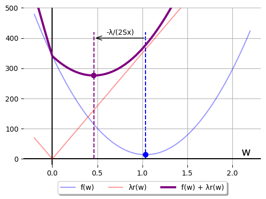
Neither \(f\) nor \(r\) are minimized at that points where they intersect the purple
vertex axis of symmetry. Both could be much smaller, if they didn't have to
accommodate the other. That's a good compromise: one that leaves everyone
angry.
Lots of regularization
When we ramp up our value of \(\lambda\) from 350 to 800 on our blue-dots example,
nothing about the rules change for our little-guy optimizer. What does change
is the layout of the two parabolae: now, neither parabola's vertex lies on the
side its rule governs:
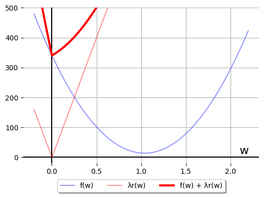
The thought process for our little guy is:
- "When I'm on the LHS, it wants me to go to
\(\left(2D_{xy} + \lambda\right)/(2S_x)\), which is on the RHS."
- "But then when I get to the RHS, it wants me to go look for a minimum at
\(\left(2D_{xy} - \lambda\right)/(2S_x)\), which is back on the LHS.
I just came from there!!"
For some optimizers, this bouncing back and forth can take awhile to resolve.
But when it does resolve, it can only end at \(w^*(800) = 0\), the maximally
simple model weight.
When does this happen? It happens when both the LHS and RHS parabolae have
vertices centered on the opposite side. This can happen no matter the sign of
\(D_{xy}\), so long as \(\lambda\) is big enough.
We can combine these two criteria -- "if \(D_{xy}\) is positive, double it" and
"if \(D_{xy}\) is negative, negate it, then double it" -- into one rule that
determines when our minimum will be at \(w = 0\):
$$\lambda > 2|D_{xy}|$$
This is the magic threshold for Lasso. Past this level of regularization,
we can only get the empty model out of the optimization.
Checking my work: in the blue-dot case, \(D_{xy} = 314.7\), and the
"Regularization Path" figure shows that \(w^*(\lambda)\) hits zero right where we
expect, around \(2 \times 314.7 = 629.4 \approx 630\).
It's good to know Lasso has this magic threshold: often we will tune the
regularization parameter so that we can find a model that works well on held-out
test data. With this magic threshold, we can put an upper bound on our search
space: past \(2|D_{xy}|\), we will always get the same zero-model result. We
don't need to keep searching past that threshold value. That's useful!
Why's Lasso do that? (Discontinuous slope.)
The slope of our Lasso objective looks like:
$$\begin{align}\frac{d}{dw}\left\{f(w) + \lambda r(w)\right\} &= \frac{d}{dw}f(w) + \lambda\frac{d}{dw}\left|w\right| \\
&= \frac{d}{dw}\left\{S_xw^2 - 2D_{xy}w + S_y\right\} + + \lambda\frac{d}{dw}\left|w\right| \\
&= 2S_xw - 2D_{xy} + \lambda\frac{d}{dw}\left|w\right| \end{align}$$
Note that part and parcel of Lasso's convexity means this slope is never
decreasing. In this univariate case, that's the definition of a convex
function, which we know Lasso to be.
The derivative for our regularizer hits a snag at \(w = 0\); the slope tangent
to \(|w|\) depends on whether you mean "sloping in from the LHS" or "sloping in
from the RHS":
$$\lambda\frac{d}{dw}|w| = \begin{cases}
-\lambda&\text{if}~w < 0 \\
\mbox{undefined}&\text{if}~w = 0 \\
\lambda&\text{if}~w > 0
\end{cases}$$
$$\frac{d}{dw}\left\{f(w) + \lambda r(w)\right\} = \begin{cases}
2S_xw - 2D_{xy} - \lambda&\text{if}~w < 0 \\
\mbox{undefined}&\text{if}~w = 0 \\
2S_xw - 2D_{xy} + \lambda&\text{if}~w > 0
\end{cases}$$
We can plot this for the zero-, some-, and lots-of-regularization models fit to
the blue-dot data, where we see a steadily larger discontinutiy at \(w = 0\):
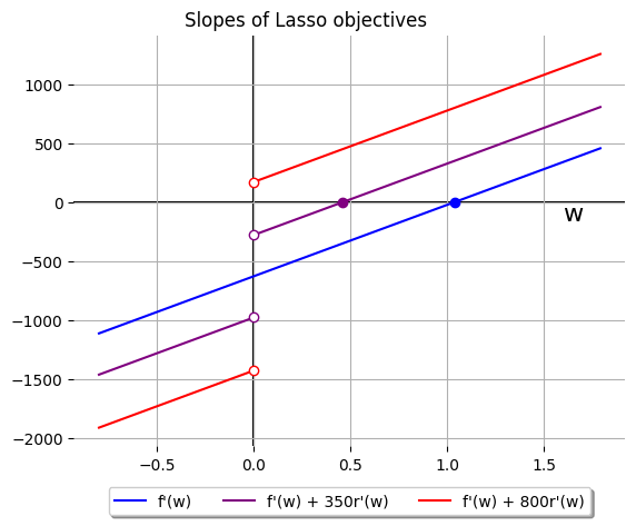
(Side note: in an alternate case where \(D_{xy}\) is negative, this plot of
slopes will look very similar. Lasso is still convex, so these slope curves
must still all be non-decreasing. The difference would be that the blue and
purple vertical-axis-intercepts would be positive instead of negative.)
For zero- and some-regularization, the blue and purple lines, we see
intersection with the horizontal axis at the same points we see the vertices of
their respective parabolae above: \(w\) values where our Lasso objective has
zero slope.
But with lots-of-regularization, there's no similar intersection. The
discontinuity introduced by \(\lambda r(w)\) is large enough
that, at \(w = 0\), the slope jumps straight from "very negative" to "slightly
positive." This pseudo-intersection with the horizontal axis determines where
our little-guy optimizer halts, just like the genuine points of zero slope in
the blue and purple models.
Looking at the slope discontinuity explains Lasso's magic threshold
\(\lambda > 2|D_{xy}|\) in a way that generalizes to other loss functions for \(f\).
The regularizer is acting like a kind of crowbar, chiseled into the
unregularized objective at the point \((w, f'(w))\), and prying the LHS and RHS
apart from each other by an additive factor of \(\lambda\).
Our blue slope line has a non-zero value at \(w = 0\). For \(\lambda|w|\) to
introduce a sign change in the slope, it either needs to push a positive \(f'(0)\)
below the horizontal axis, or (as in the blue-dots example here) push a negative
\(f'(0)\) above the horizontal axis. As in, we get the maximally-simple model
whenever we set:
$$\lambda \geq \left|f'(0)\right|$$
For original-recipe Lasso, where our loss \(f\) is the ordinary least squares
function, \(f'(0) = 2D_{xy}\). Plug that in above and recover the magic
threshold. Without any regularization (for \(D_{xy} > 0\) here, but the logic
holds in the mirror case, too), \(f(w)\) decreases as you move from \(w = 0\) into
the RHS. Even with some regularization, \(f(w) + \lambda r(w)\) decreases as
you move into the RHS -- it has a negative slope at \(w = 0^+\).
In sum,
- The function we're optimizing is convex, so its slope is non-decreasing. If
out little guy is ever at a point where the slope is negative, it must move
right to hope to reach a minimum where the slope is zero. And if it's ever
at a point of positive slope, it must move left.
- With the discontinuity of Lasso's regularizer, we see two different slopes at
\(w = 0\), depending if we approach 0 from the LHS or the RHS.
- When \(\lambda\) is big enough, relative to the slope \(f'(0)\), these two slopes
will have opposite signs. The sign of
\(\left[f'(-\epsilon) + \lambda r(-\epsilon)\right]\) will be negative, and the
sign of \(\left[f'(-\epsilon) + \lambda r(-\epsilon)\right]\) will be positive,
for any \(\epsilon > 0\).
- And so we get stuck right at \(w = 0\). Try to move a bit left off zero,
to \(w = 0^-\), and you will sense a negative slope, and get told to move back
right. Try to move a bit right, to \(w = 0^+\), and get told to move back
left.
- The little guy optimizer gets driven to \(w = 0\) itself, and can't go anywhere
else.
That's why Lasso does that.
Returning to multiple features
This same phenomenon applies even when we reinflate from \(p = 1\) univariate
feature, back to the \(p > 1\) multivariate case. Lasso does this in high
dimensions, too.
Bringing back our original \(N\) vector-scalar pairs,
\(\left\{\vec{\mathbb{x}}_j, y_j\right\}_{j = 1}^N\), I'm going to define some
new helper aliases. First, imagine stacking all the feature vectors,
transposed horizontally, into a matrix
\(\mathbf{X} \in \mathbb{R}^{N \times p}\):
$$\mathbf{X} = \left[\begin{array}{c} ~~- \vec{\mathbb{x}}_1^T -~~ \\
\vdots \\
~~- \vec{\mathbb{x}}_j^T -~~ \\
\vdots \\
~~- \vec{\mathbb{x}}_N^T -~~ \\
\end{array}\right]$$
Now imagine pulling out the \(i\)th column from that matrix: it encodes the
\(i\)th predictive feature for each datum \(j = 1, \ldots, N\). Call each of these
column vectors \(\vec{\mathbb{x}}^{(i)} \in \mathbb{R}^N\), \(i = 1, \ldots, p\):
$$\mathbf{X} = \left[\begin{array}{c} ~~- \vec{\mathbb{x}}_1^T -~~ \\
\vdots \\
~~- \vec{\mathbb{x}}_j^T -~~ \\
\vdots \\
~~- \vec{\mathbb{x}}_N^T -~~ \\
\end{array}\right] = \left[\begin{array}{ccccc}
\vert & & \vert & & \vert \\
\vec{\mathbb{x}}^{(1)} & \cdots & \vec{\mathbb{x}}^{(i)} & \cdots & \vec{\mathbb{x}}^{(p)} \\
\vert & & \vert & & \vert \\
\end{array}\right]$$
And let's also pull the labels \(y_j\) into their own column vector:
$$\vec{\mathbb{y}} = \left[\begin{array}{c} y_1 \\
\vdots \\
y_N
\end{array}\right] \in \mathbb{R}^N$$
Imagine, for our multivariate dataset, we have currently set our little-guy
optimizer at the fully sparse, all-zeros weight vector,
\(\vec{\mathbb{w}} = \vec{\mathbb{0}}\). What would it take to convince the
little guy to move any single model weight off of zero?
The little guy can consider each feature, \(\vec{\mathbb{x}}^{(i)}\), one at a
time, as if each were its own individual univariate Lasso case. The current
weight vector ignores every feature, so the question of "should we put any
weight on feature \(i\)?" depends only on the univariate dataset
\(\left\{\vec{\mathbb{x}}^{(i)}_j, y_j\right\}_{j=1}^N\); the other features are
currently zeroed out and of no concern.
For feature \(i\), the magic threshold is the analogue of \(2|D_{xy}|\), taking a
dot product between the \(i\)th feature column vector and the label column vector:
$$\lambda > 2\left|\vec{\mathbb{y}}^T\vec{\mathbb{x}}^{(i)}\right|$$
The little guy will not move off \(\vec{\mathbb{w}} = \vec{\mathbb{0}}\) if
\(\lambda\) is big enough to cross the magic threshold for all \(p\) features.
Which means have a meta-magic threshold in the multivariate case that zeros
out all \(p\) model weights, just by ramping \(\lambda\) to a big enough value:
$$\lambda > \max_{i = 1, \ldots, p}2\left|\vec{\mathbb{y}}^T\vec{\mathbb{x}}^{(i)}\right|
\Rightarrow \vec{\mathbb{w}}^*(\lambda) = \vec{\mathbb{0}}$$
(Note that the \(\max_i\) operation is the same as, for our definition of matrix
\(\mathbf{X}\) above: "calculate the vector
\(\mathbf{X}^T\vec{\mathbb{y}}\), then find the largest-magnitude element.")
This is also good to know! If we're using crossvalidation to hunt for the
perfect \(\lambda\) parameter, it continues to be nice to have an upper bound on
the search space. It's good to understand why a statistical technique works.